Vanishing Points in Homogeneous Coordinates

By Esther Ling

Introduction

We know that train tracks form parallel lines. However, in a thought experiment, if we were to stand on the tracks and observe the two outer rails, they would appear to meet as our glance approaches the horizon. Due to perspective projection, these parallel lines converge at a point called the vanishing point, or, the point at infinity [1]. In this post, I explore the use of homogeneous coordinates for reasoning about the intersection of parallel lines.

Homogeneous Coordinates

Homogeneous coordinates is a coordinate system used in projective geometry. Contrast this with the Cartesian coordinate system for Euclidean geometry. In computer vision, where we deal with projections from our 3D world to the 2D image plane, it is useful to be able to operate in either coordinate system. One way to think about homogeneous coordinates is that they are used to express points from \(\mathbb{R}^d\) in \(\mathbb{R}^{d+1}\) space, by augmenting a 1 for the added dimension.

Points

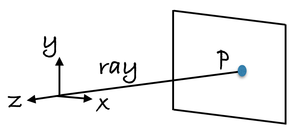
A point \(p \in \mathbb{R}^2\) in the image plane can be thought of as a ray in 3D space.

When a 3D world point \(P \in \mathbb{R}^3\) is projected onto the image plane, the depth information is lost. Consequently, when we want to figure out which world point caused \(p\), we only know the answer up to scale. In other words, each point \(p\) is mapped not to a single point \(P\), but an equivalence class of points.

So, every point on the image plane can be thought of as a ray in 3D space. Is there a way of representing a point in the image plane, such that it captures the notion of “3D-ness” (i.e. the ray from which it originates)? Using homogeneous coordinates! - we express \(p \in \mathbb{R}^2\) as \(\tilde{p} \in \mathbb{R}^{2+1} = \mathbb{R}^{3}\).

Define our image point in homogeneous coordinates as:

\(\tilde{p} = [x, y, 1]^T\).

To convert back to Euclidean coordinates from homogeneous coordinates, we divide the first and second element by the third element:

\(p = [x/z, y/z]^T\).

Looking at the diagram again, notice that any point along the ray is equivalent to another point on that ray, which this representation captures:

for some \(\alpha \in \mathbb{R}\) to represent the possible depths where the 3D point lies.

Notice that we can also express the ray in 3D space as a line: \(r = [a, b, c]^T\).

With this representation, we are able to express points in the image and their rays in the same coordinate system.

Lines

How about lines in an image?

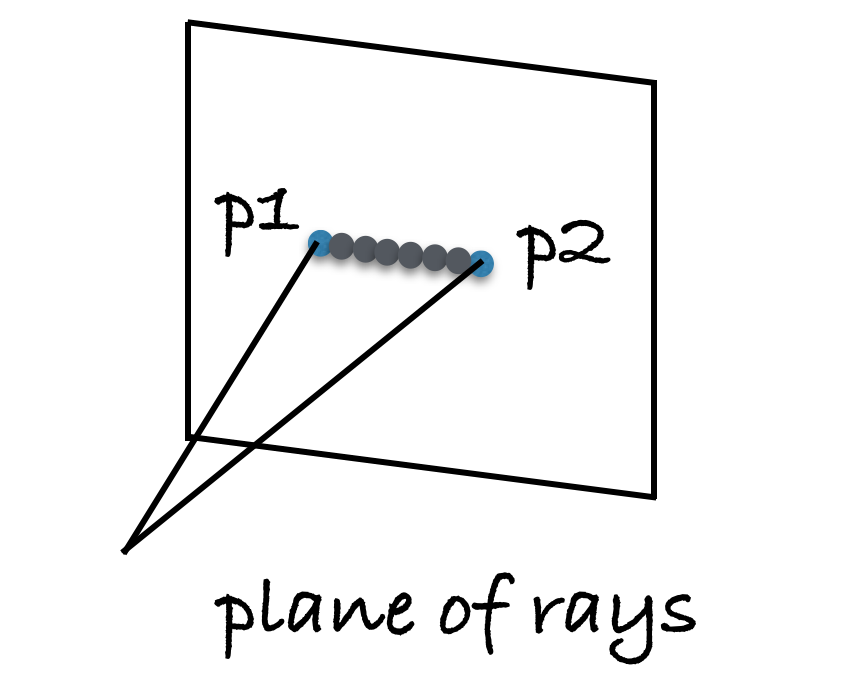
We can think of a line as having two end points, with infinitely many points in between them. Each of these points have a ray associated with them. So, a line in an image forms a plane in 3D space.

We can parametrize a line in the image using homogeneous coordinates by \(l = [a, b, c]^T\), where \(ax + by + cz = 0\).

To relate this system with how we might be more familiar with parameterizing lines (i.e. a slope and an intercept):

Sub-in point \(\tilde{p} = [x, y, 1]^T\) into the equation above, to get:

\(ax + by + c = 0\).

Re-arranging, we get:

where the slope = \(-\frac{a}{b}\) and the intercept = \(-\frac{c}{b}\).

Intersection of Lines

Generally, two lines \(l_1\) and \(l_2\) intersect at a point \(k\).

With the slope and intercept line parameterization, we can find this point by equating the equations for \(l_1\) and \(l_2\):

to find \(k = [x, y]^T\).

However, we run into a problem when the slopes are equivalent, i.e. \(m_1 = m_2\). In other words, the slope and intercept line parameterization doesn’t really help us when thinking about the intersection of two parallel lines.

Let’s see if homogeneous coordinates are more helpful.

Theorem:

The intersection point \(\tilde{k}\) between two lines \(l_1\) and \(l_2\) can be found by \(\tilde{k} = l_1 \times l_2\), where \(\times\) denotes the vector cross-product.

Proof:

If \(l_1\) and \(l_2\) intersect, then the intersection point \(\tilde{k}\) falls on both lines. Then, we just need to show that \(l_1^T\tilde{k}=0\) and \(l_2^T\tilde{k}=0\) are true. From the statement \(\tilde{k} = l_1 \times l_2\), \(\tilde{k}\) is a vector orthogonal to the space spanned by \(l_1\) and \(l_2\). Hence, \(l_1^T\tilde{k}=0\) and \(l_2^T\tilde{k}=0\) are true. q.e.d.

Suppose \(l_1\) and \(l_2\) are parallel. Then, they have the same slope:

Using the cross-product to find their intersection:

Now, when we convert \(\tilde{k}\) back to its Euclidean form, we get:

which is a division by zero, and hence a point at infinity!

Parallel Lines with Equal Slope Meet

We can extend the analysis to show that all lines parallel to \(l_1\) and \(l_2\) intersect at the same point \(k_\infty\).

First, we can simplify \(\tilde{k}\)

where \(\alpha = c_2 - c_1\).

Let \(l_p\) represent any line parallel to \(l_1\) and \(l_2\), i.e

\(l_p = [a, b, c_p]^T\).

What remains to show is \(l_p^T k_\infty = 0\).

Expanding \(l_p^T k_\infty\):

\(l_p^T k_\infty = \left[ \begin{array}{ccc} a & b & c \end{array} \right]\left[ \begin{array}{c} b \\ -a \\ 0 \end{array} \right] = 0\).

Hence, any line parallel to \(l_1\) and \(l_2\) intersect at the same point \(k_\infty\).

References

[1] I came across this illustration in the book “How not to be wrong - the power of mathematical thinking” by Jordan Ellenberg.

[2] I credit much of the math in this piece to these course notes.